Excel Data Analysis 简明教程
Excel Data Analysis - Data Validation
数据验证是 Excel 中一个非常有用、易于使用的工具,使用它可以在输入工作表的数据上设置数据验证。
Data Validation is a very useful and easy to use tool in Excel with which you can set data validations on the data that is entered that is entered into your Worksheet.
对于工作表上的任何单元格,您都可以
For any cell on the worksheet, you can
-
Display an input message on what needs to be entered into it.
-
Restrict the values that get entered.
-
Provide a list of values to choose from.
-
Display an error message and reject an invalid data entry.
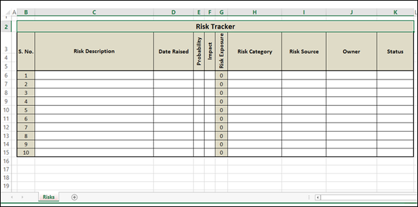
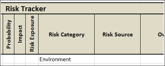
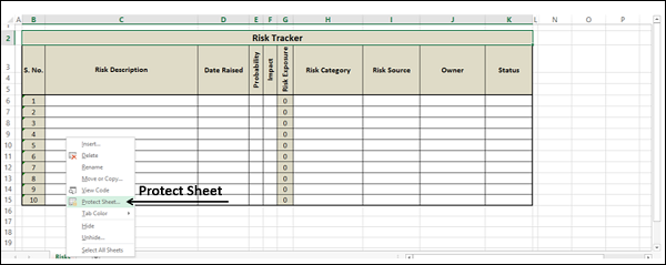
考虑以下风险跟踪器,该跟踪器可用于输入和跟踪已识别的风险信息。
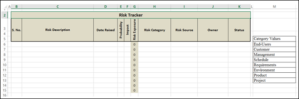
Consider the following Risk Tracker that can be used to enter and track the identified Risks information.
在此跟踪器中,输入以下列中的数据的验证采用预设数据约束,并且仅当输入的数据满足验证标准时才会接受。否则,您将收到一条错误消息。
In this tracker, the data that is entered into the following columns is validated with preset data constraints and the entered data is accepted only when it meets the validation criteria. Otherwise, you will get an error message.
-
Probability
-
Impact
-
Risk Category
-
Risk Source
-
Status
“风险敞口”列将具有计算值,您不能输入任何数据。甚至连 S. No. 列都设置为具有计算值,即使您删除了一行,这些计算值也会进行调整。
The column Risk Exposure will have calculated values and you cannot enter any data. Even the column S. No. is set to have calculated values that are adjusted even if you delete a row.
现在,您将学习如何设置这样的工作表。
Now, you will learn how to set up such a worksheet.
Prepare the Structure for the Worksheet
为工作表的结构做准备 −
To prepare the structure for the worksheet −
-
Start with a blank worksheet.
-
Put the header in Row 2.
-
Put the column headers in Row 3.
-
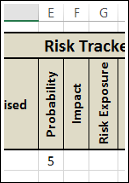
For the column headers Probability, Impact and Risk Exposure − Right click on the cell.Click on Format Cells from drop down.In the Format Cells dialog box, click on Alignment tab.Type 90 under Orientation.
-
Merge and Centre the cells in Rows 3, 4, and 5 for each of the column headers.
-
Format Borders for the cells in Rows 2 – 5.
-
Adjust the row and column widths.
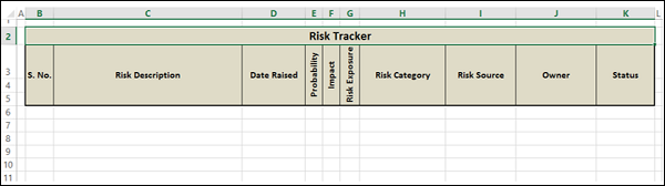
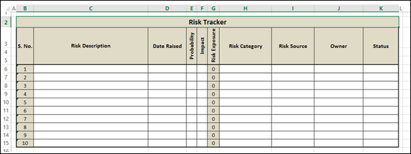
您的工作表将如下所示 −
Your worksheet will look as follow −
Set Valid Values for Risk Category
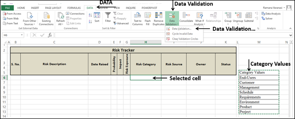
在 M5 - M13 单元格中输入以下值(M5 为标题,M6 - M13 为值)
In the cells M5 – M13 enter the following values (M5 is heading and M6 - M13 are the values)
Category Values |
End-Users |
Customer |
Management |
Schedule |
Schedule |
Environment |
Product |
Project |
-
Click the first cell under the column Risk Category (H6).
-
Click DATA tab on the Ribbon.
-
Click Data Validation in the Data Tools group.
-
Select Data Validation… from the drop-down list.
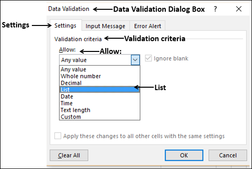
数据验证对话框出现。
The Data Validation dialog box appears.
-
Click the Settings tab.
-
Under Validation criteria, in the Allow: drop-down list, Select the option List.
-
Select the range M6:M13 in the Source: box that appears.
-
Check the boxes Ignore blank and In-cell dropdown that appear.

Set Input Message for Risk Category
-
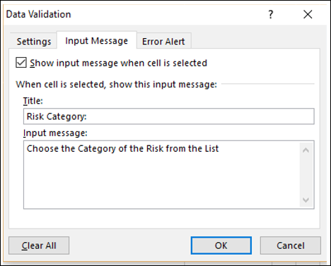
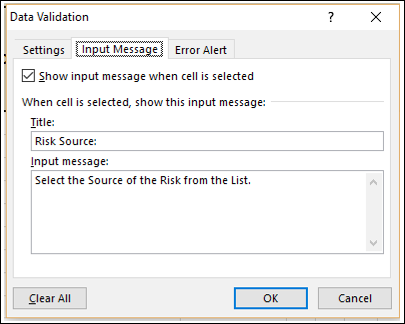
Click the Input Message tab in the Data Validation dialog box.
-
Check the box Show input message when cell is selected.
-
In the box under Title:, type Risk Category:
-
In the box under Input message: Choose the Category of the Risk from the List.
Set Error Alert for Risk Category
要设置错误警报,请执行以下操作:
To set error alert −
-
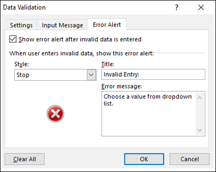
Click the Error Alert tab in the Data validation dialog box.
-
Check the box Show error alert after invalid data is entered.
-
Select Stop under Style: dropdown
-
In the box under Title:, type Invalid Entry:
-
In the box under Error message: type Choose a value from dropdown list.
-
Click OK.
Verify Data Validation for Risk Category
对于风险类别下的选定的第一个单元格,
For the selected first cell under Risk Category,
-
Data Validation criteria is set
-
Input message is set
-
Error alert is set
现在,您可以验证设置。
Now, you can verify your settings.
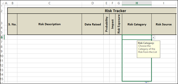
单击您已针对其设置数据验证条件的单元格。此时,将显示“输入”消息。“下拉”按钮将出现在单元格右侧。
Click in the cell for which you have set Data Validation criteria. The Input message appears. The dropdown button appears on the right side of the cell.
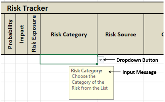
“输入”消息显示正确。
The input message is correctly displayed.
-
Click on the dropdown button on the right side of the cell. The drop-down list appears with the values that can be selected.
-
Cross-check the values in the drop-down list with those that are used to create the drop-down list.
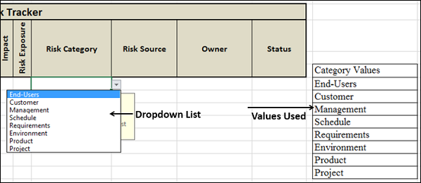
两组值相匹配。请注意,如果值的数量更多,则您将在下拉列表的右侧看到一个向下滚动条。
Both the sets of values match. Note that if the number of values is more, you will get a scroll-down bar on the right side of the dropdown list.
从下拉列表中选择一个值。它将显示在单元格中。
Select a value from the dropdown list. It appears in the cell.
您可以看到合法值的选择工作正常。
You can see that the selection of valid values is working fine.
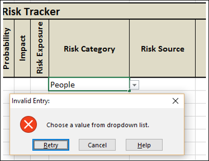
最后,尝试输入无效项并验证错误警报。
Finally, try to enter an invalid entry and verify the Error alert.
在单元格中键入 People,然后按 Enter。系统将显示您为该单元格设置的错误消息。
Type People in the cell and press Enter. Error message that you have set for the cell will be displayed.
-
Verify the Error message.
-
You have an option to either Retry or Cancel. Verify both the options.
您已成功为该单元格设置了数据验证。
You have successfully set the Data Validation for the cell.
Note − 查看您消息的拼写和语法非常重要。
Note − It is very important to check the spelling and grammar of your messages.
Set Valid Criteria for the Risk Category Column
现在,您可以对风险类别列中的所有单元格应用数据验证条件。
Now, you are ready to apply the Data Validation criteria to all the cells in the Risk Category column.
此时,您需要记住两件事 −
At this point, you need to remember two things −
-
You need to set the criteria for maximum number of cells that are possible to be used. In our example, it can vary from 10 – 100 based on where the worksheet will be used.
-
You should not set the criteria for unwanted range of cells or for the entire column. This will unnecessarily increases the file size. It is called excess formatting. If you get a worksheet from an outside source, you have to remove the excess formatting, which you will learn in the chapter on Inquire in this tutorial.
按照以下步骤操作 −
Follow the steps given below −
-
Set the validation criteria for 10 cells under Risk Category.
-
You can easily do this by clicking on the right-bottom corner of the first cell.
-
Hold on the + symbol that appears and pull it down.
数据验证被设置为所有选中的单元格。
Data Validation is set for all the selected cells.
单击被选中的最后一列并验证。
Click the last column that is selected and verify.
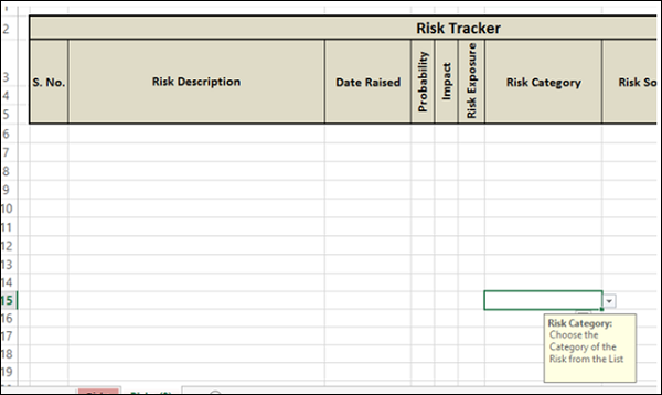
风险类别列的数据验证已完成。
Data Validation for the column Risk Category is complete.
Set Validation Values for Risk Source
在这种情况下,我们只有两个值——内部和外部。
In this case, we have only two values – Internal and External.
-
Click in the first cell under the column Risk Source (I6)
-
Click the DATA tab on the Ribbon
-
Click Data Validation in the Data Tools group
-
Select Data Validation… from the drop-down list.
将出现数据验证对话框。
Data Validation dialog box appears.
-
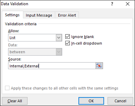
Click the Settings tab.
-
Under Validation criteria, in the Allow: drop-down list, select the option List.
-
Type Internal, External in the Source: box that appears.
-
Check the boxes Ignore blank and In-cell dropdown that appear.
设置风险来源的输入消息。
Set Input Message for Risk Source.
设置风险来源的错误警报。
Set Error Alert for Risk Source.
对于风险来源下的选定的第一个单元格 -
For the selected first cell under Risk Source −
-
Data Validation criteria is set
-
Input message is set
-
Error alert is set
现在,您可以验证设置。
Now, you can verify your settings.
单击您已为其设置数据验证条件的单元格。将出现输入消息。下拉按钮将出现在单元格的右侧。
Click in the cell for which you have set Data Validation criteria. Input message appears. The drop-down button appears on the right side of the cell.
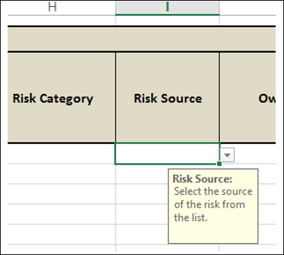
输入消息正确显示。
The input message is displayed correctly.
-
Click the drop-down arrow button on the right side of the cell. A drop-down list appears with the values that can be selected.
-
Check if the values are the same as you typed – Internal and External.

这两组值都匹配。从下拉列表中选择一个值。该值将出现在单元格中。
Both the sets of values match. Select a value from the drop-down list. It appears in the cell.
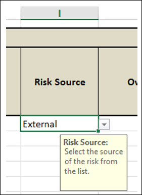
你可以看到,有效值的选定正常工作。最后,尝试输入一个无效的条目并核实错误警告。
You can see that the selection of valid values is working fine. Finally, try to enter an invalid entry and verify the Error alert.
在单元格中键入财务并按 Enter。你会看到设置到该单元格的错误消息。
Type Financial in the cell and press Enter. Error message that you have set for the cell will be displayed.

-
Verify the Error message. You have successfully set the Data Validation for the cell.
-
Set valid criteria for the Risk Source Column
-
Apply the Data Validation criteria to the cells I6 - I15 in the Risk Source column (i.e. same range as that of Risk Category column).
数据验证已设置到所有所选单元格。数据验证已针对风险来源列完成。
Data Validation is set for all the selected cells. Data Validation for the column Risk Source is complete.
Set Validation Values for Status
-
Repeat the same steps that you used for setting Validation values for Risk Source.
-
Set the List values as Open, Closed.
-
Apply the Data Validation criteria to the cells K6 - K15 in the Status column (i.e. same range as that of Risk Category column).
数据验证已设置到所有所选单元格。数据验证已针对状态列完成。
Data Validation is set for all the selected cells. Data Validation for the column status is complete.
Set Validation Values for Probability
风险概率分数值在范围 1-5 内,1 为低,5 为高。此值可以是 1 和 5 之间的任意整数(包括 1 和 5)。
Risk Probability Score values are in the range 1-5, 1 being low and 5 being high. The value can be any integer between 1 and 5, both inclusive.
-
Click in the first cell under the column Risk Source (I6).
-
Click the DATA tab on the Ribbon.
-
Click Data Validation in the Data Tools group.
-
Select Data Validation… from the drop-down list.
数据验证对话框出现。
The Data Validation dialog box appears.
-
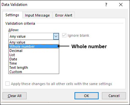
Click the Settings tab.
-
Under Validation criteria, in the Allow: drop-down list, select Whole number.
-
Select between under Data:
-
Type 1 in the box under Minimum:
-
Type 5 in the box under Maximum:

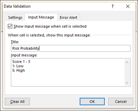
设置概率的输入消息
Set Input Message for Probability
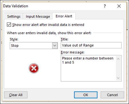
设置概率的错误警告并点击确定。
Set Error Alert for Probability and click OK.
对于概率下的第一个所选单元格,
For the selected first cell under Probability,
-
Data Validation criteria is set.
-
Input message is set.
-
Error alert is set.
现在,您可以验证设置。
Now, you can verify your settings.
点击已设置数据验证准则的单元格。出现输入信息。在这种情况下,不会有下拉按钮,因为输入值被设置为在一个范围内,而非一个列表中。
Click on the cell for which you have set Data Validation criteria. Input message appears. In this case, there will not be a dropdown button because the input values are set to be in a range and not from list.
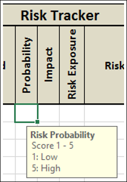
“输入”消息显示正确。
The input message is correctly displayed.
在单元格中输入介于 1 和 5 之间的整数。它会出现在单元格中。
Enter an integer between 1 and 5 in the cell. It appears in the cell.
有效值的选取工作正常。最后,尝试输入一个无效项,并验证错误警告。
Selection of valid values is working fine. Finally, try to enter an invalid entry and verify the Error alert.
在单元格中键入 6,然后按 Enter。将显示为该单元格设置的错误消息。
Type 6 in the cell and press Enter. The Error message that you have set for the cell will be displayed.

您已成功为该单元格设置了数据验证。
You have successfully set the Data Validation for the cell.
-
Set valid criteria for the Probability Column.
-
Apply the Data Validation criteria to the cells E6 - E15 in the Probability column (i.e. same range as that of Risk Category column).
已为所有选定的单元格设置了数据验证。列“可能性”的数据验证完成。
Data Validation is set for all the selected cells. Data Validation for the column Probability is complete.
Set Validation Values for Impact
若要设置影响的验证值,请重复为设置可能性的验证值所用的相同步骤。
To set the validation values for Impact, repeat the same steps that you used for setting validation values for probability.
将数据验证准则应用于“影响”列中的单元格 F6 - F15(即与“风险类别”列相同的范围)。
Apply the Data Validation criteria to the cells F6 - F15 in the Impact column (i.e. same range as that of Risk Category column).
已为所有选定的单元格设置了数据验证。列“影响”的数据验证完成。
Data Validation is set for all the selected cells. Data Validation for the column Impact is complete.
Set the Column Risk Exposure with Calculated Values
风险暴露被计算为风险可能性和风险影响的乘积。
Risk Exposure is calculated as a product of Risk Probability and Risk Impact.
风险暴露 = 可能性 * 影响
Risk Exposure = Probability * Impact
在单元格 G6 中键入 =E6*F6,然后按 Enter。
Type =E6*F6 in cell G6 and press Enter.
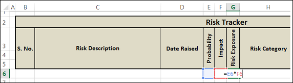
由于 E6 和 F6 为空,因此单元格 G6 中将显示 0。
0 will be displayed in the cell G6 as E6 and F6 are empty.
将公式复制到单元格 G6 – G15 中。单元格 G6 - G15 中将显示 0。
Copy the formula in the cells G6 – G15. 0 will be displayed in the cells G6 - G15.
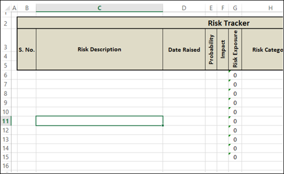
由于“风险暴露”列用于计算值,因此你不应允许在该列中输入数据。
As the Risk Exposure column is meant for calculated values, you should not allow data entry in that column.
-
Select cells G6-G15
-
Right-click and in the dropdown list that appears, select Format Cells. The Format Cells dialog box appears.
-
Click the Protection tab.
-
Check the option Locked.
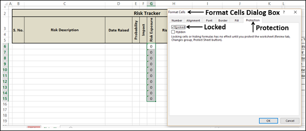
这是为了确保不允许在那些单元格中输入数据。不过,只有在工作表受保护后,这才会生效。工作表准备好后,你将作为最后一步执行此操作。
This is to ensure that data entry is not allowed in those cells. However, this will come into effect only when the worksheet is protected, which you will do as the last step after the worksheet is ready.
-
Click OK.
-
Shade the cells G6-G15 to indicate they are calculated values.
Format Serial Number Values
你可以让用户自己填写序号列。但是,如果你对序号值进行格式化,那么工作表看起来会更美观。此外,它还可以显示工作表格式化了多少行。
You can leave it to the user to fill in the S. No. Column. However, if you format the S. No. values, the worksheet looks more presentable. In addition, it shows for how many rows the worksheet is formatted.
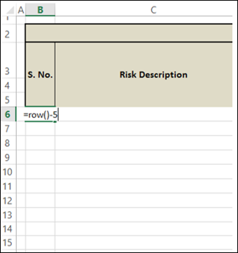
在单元格 B6 中输入 =row()-5,然后按 Enter 键。
Type =row()-5 in the cell B6 and press Enter.
1 会显示在单元格 B6 中。将此公式复制到单元格 B6-B15 中。会显示值 1-10。
1 will appear in cell B6. Copy the formula in the cells B6-B15. Values 1-10 appear.
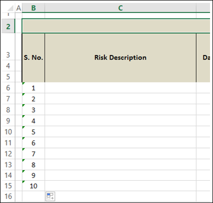
对单元格 B6-B15 进行阴影填充。
Shade the cells B6-B15.
Wrap-up
你的项目几乎就完成了。
You are almost done with your project.
-
Hide Column M that contains Data Category values.
-
Format Borders for the cells B6-K16.
-
Right-click on the worksheet tab.
-
Select Protect Sheet from the menu.
“保护工作表”对话框随即显示。
The Protect Sheet dialog box appears.
-
Check the option Protect worksheet and contents of locked cells.
-
Type in a password under Password to unprotect sheet − Password is case sensitiveProtected sheet cannot be recovered if password is forgottenIt is a good practice to keep a list of worksheet names and passwords somewhere
-
Under Allow all users of this worksheet to: check the box Select unlocked cells.
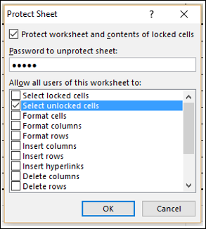
你已将列“风险敞口”中的锁定单元格受保护,不准录入数据,并将其余的解锁单元格保持为可编辑状态。单击“确定”。
You have protected the locked cells in the column Risk Exposure from data entry and kept the rest of the unlocked cells editable. Click OK.
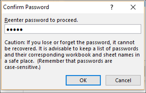
“ Confirm Password ”对话框显示。
The Confirm Password dialog box appears.
-
Re-enter the password.
-
Click OK.
已设置好数据验证的单元格的工作表可以使用了。
Your worksheet with Data Validation set for selected cells is ready to use.